Table of Contents
6.1 Motivation and outline: How to deal with constraint motion?
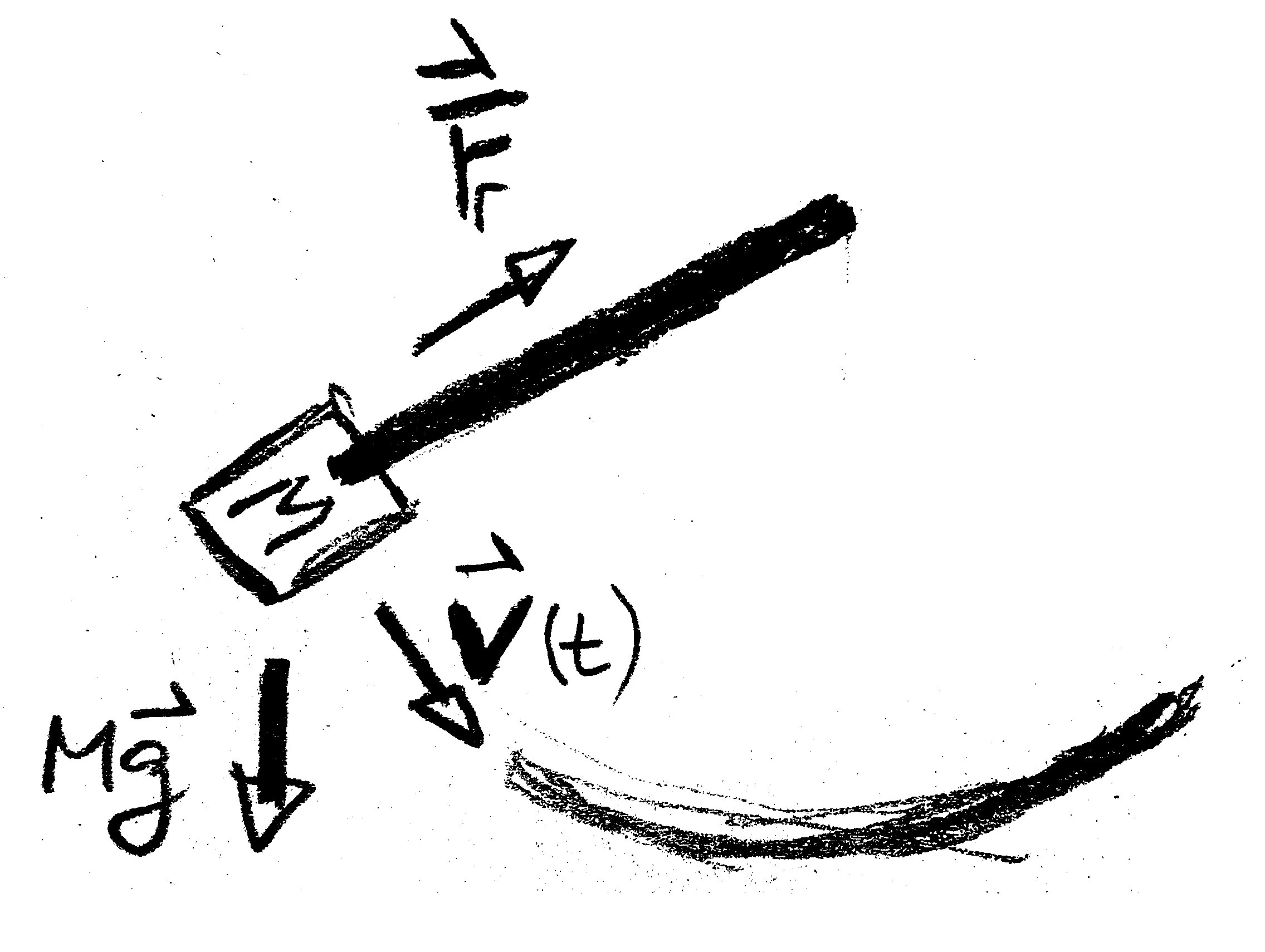
 Figure 6.2: Forces acting for the motion of a swing, or its equivalent idealization of of a mathematical pendulum.
Almost all interesting problems in mechanics involve constraints due to rails or tracks, and due to mechanical joints of particles. The most elementary example is a swing (Figure 6.1), where a rope forces a mass $M$ to move on a path with positions constrained to a circle with radius given by the length $L$ of the rope. Gravity $M \, \mathbf g$ and the pulling force $\mathbf F_r$ of the rope acting act on the mass (Figure 6.2). However, how large is the latter force? At the topmost point of its trajectory the mass is at rest, and no force is needed along the rope to keep it on its track. At the lowermost point, where the swing goes with its maximum speed, there is a substantial force. Newton's formalism requires a discussion of these forces. Lagrange established an alternative approach that provides equations of motion with substantially less effort. The key idea of this formalism is to select generalized coordinates adapted to the problem.
Definition 6.1 Generalized Coordinates
We consider $N$ particles moving in $D$ dimensions.
There are forces that keep the particles on a subset of space with a dimension smaller than $D$,
and their relative positions may be constrained by bars and joints.
Due to the constrains the system only has $M < D \, N$ degrees of freedom.
In this chapter we denote the positions of the particles as
$\mathbf x \in \mathbb{R}^{D\,N}$,
and we specify position compatible with the constraints
as $\mathbf x( \mathbf q(t) )$,
where $\mathbf q \in \mathbb{R}^{M}$
are the generalized coordinates
adapted to the constrained motion.
Example 6.1 Generalized coordinates for a pendulum
We describe the position of the mass in a mathematical pendulum by the angle $\theta(t)$,
as introduced in Example 1.10.
The position of the mass in the 2D pendulum plane is thus described by the vector
\begin{align*}
\mathbf x(t)
= L \begin{pmatrix} \sin\theta(t) \\ -\cos\theta(t) \end{pmatrix}
= L \, \hat{\mathbf R}(\theta(t)) \, .
\end{align*}
In view of the chain rule its velocity amounts to
\begin{align*}
\dot{\mathbf x}
&= L \, \dot\theta \: \partial_\theta \hat{\mathbf R}(\theta(t))
= L \, \dot\theta \: \hat{\boldsymbol\theta}(\theta(t))
\quad
\text{with }
\hat{\boldsymbol\theta}(\theta(t)) = \begin{pmatrix} \cos\theta(t) \\ \sin\theta(t) \end{pmatrix}
\end{align*}
Remark 6.1. Note that $\hat{\mathbf R}(\theta)$ and $\hat{\boldsymbol\theta}(\theta)$ are orthonormal vectors that describe the position of the mass in terms of polar coordinates rather than fixed-in-space Cartesian coordinates.
Theorem 6.1 Basis vectors for polar coordinates
Let $\{ \hat{\boldsymbol x}, \hat{\boldsymbol z}\}$ be a basis of $\mathbb R^2$, and
$(R,\theta)$ be the polar coordinates1)
associated to a point with cartesian coordinates $(x,z)$.
Then
- $R = \sqrt{x^2+z^2}$ is the distance of the point from the origin
- $\theta = -\arctan(x/z)$ the angle with respect to $-\hat{\boldsymbol z}$,
We denote the vector from the origin to $(R,\theta)$ as $R \: \hat{\boldsymbol R}(\theta)$. Then the following statements hold
- $\hat{\boldsymbol R}(\theta)$ is a normal vector at the position $(R,\theta)$ of a circle $\mathsf{C}_R$ with center at the origin at radius $R$.
- $\hat{\boldsymbol \theta} = \partial_\theta \hat{\boldsymbol R}$ is a vector tangential to $\mathsf{C}_R$ at the position $(R, \theta)$.
- $\partial_\theta \hat{\boldsymbol \theta} = - \hat{\boldsymbol R}$.
- For every $\theta \in [0, 2\pi)$ the vectors $\{ \hat{\boldsymbol R}(\theta), \hat{\boldsymbol \theta}(\theta)\}$ form an orthonormal basis of $\mathbb R^2$.
Remark 6.2. The coordinate representation of $\hat{\boldsymbol R}(\theta)$ and $\hat{\boldsymbol \theta}(\theta)$ in cartesian coordinates is provided in Example 6.2.
Remark 6.3. The assertions of Theorem 6.1 also apply when the unit vectors of $\mathbb R^2$ are denoted as $\{ \hat{\boldsymbol x}, \hat{\boldsymbol y}\}$, and when the angle $\theta$ denotes the angle with respect of the $\hat{\boldsymbol x}$ axis. The different reference axis only changes the coordinate representation of the vectors.
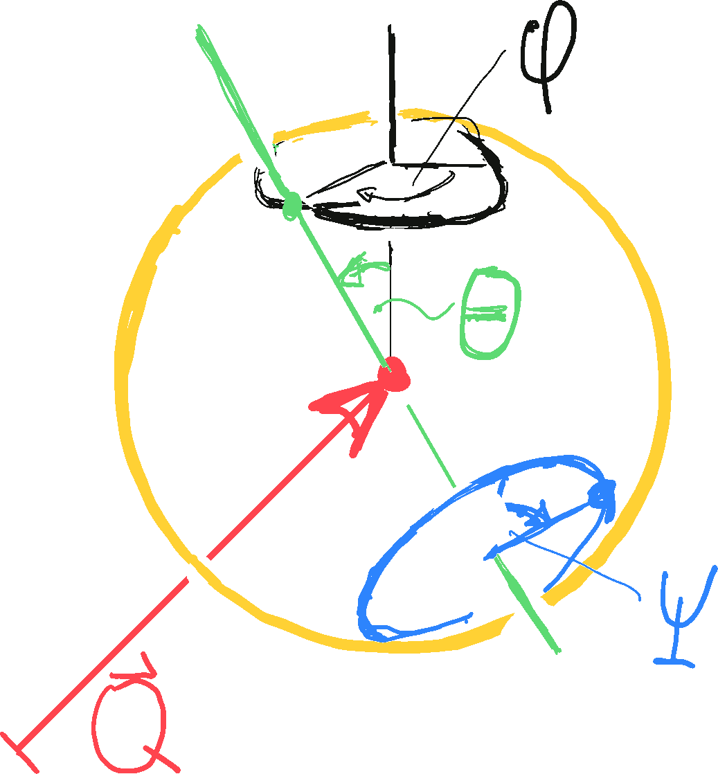
 Figure 6.3: The position of a ball in space can be described in terms of a 3D vector $\mathbf Q$ that describes the center of the ball (red dot),
angles $\theta,\phi$ that describe the orientation in space of a fixed axes in the ball (green line),
and another angle $\psi$ that describes the position of point that is not on the axis (blue point).
Example 6.2 Generalized coordinates for a ping-pong ball
A ping-pong ball consists of $N$ atoms located in the three-dimensional space.
During a match they follow an intricate trail in the vicinity of the ping-pong players.
At any time during their motion the atoms are located on a thin spherical shell with fixed positions with respect to each other.
Rather than specifying the position of each atom one can therefore specify the position of the ball in terms of six generalized coordinates (Figure 6.3):
Three coordinates provide its center of mass.
The orientation of the ball can be provided by specifying the orientation of a body fixed axis in terms of its polar and azimuthal angle,
and a third angle specifies the orientation of a point on its equator
when rotating the ball around the axis.
Generalized coordinates describe only positions complying with the constraints of the motion, and they do not account for other positions from the very beginning. Lagrange's key observation is that constraint forces, e.g., the force on the rope of the swing, only act in a direction orthogonal to the positions described by generalized coordinates. Therefore, the constraint forces do not affect the time evolution of generalized coordinates. For the pendulum and the ping-pong ball one only has to account for gravity to find the evolution of the generalized coordinates. There is no need to deal with the force along the rope in the swing, and the atomic interaction forces that keep atoms in their positions in the ping-pong ball.
Outline
In Section 6.2 we will introduce the Lagrange formalism that will allow us without much ado to determine the EOM for generalized coordinates. Subsequently, in Section 6.3 we deal with systems with a single degree of freedom. In Section 6.4 we will see how symmetries in the dynamics allow us to eliminate a second degree of freedom based on an informed choice of generalized coordinates. Section 6.5 deals with two-particle systems and other problems where one deals with several degrees of freedom. In all cases we will eventually reduce the dynamics to one-dimensional problems. The final Section 6.6 deals with the relation between continuous symmetries of the dynamics and conservation laws.
6.1.1 Self Test
Problem 6.1: Different reference axes for polar coordinates
Verify the assertions of Theorem 6.1 and Remark 6.3:
- Specify the coordinate representation of $\{ \hat{\boldsymbol R}(\theta), \hat{\boldsymbol \theta}(\theta)\}$ for the case where $\theta$ denoes the angle with respect to the positive $\hat{\boldsymbol x}$ axis.
- Verify the assertion of Theorem 6.1.
Problem 6.2: Describing the orientation of dice
We place a die on the table such that its center lies at the origin of a 3D cartesian coordinate frame,
and its axes are aligned with the coordinate axes.
We characterize the configuration of the die by the number of dots on the faces pointing in the three positive coordinate directions.
- Show that there are 24 different possibilities to place the die.
- Determine the angles $(\theta, \phi, \psi)$ (cf Figure 6.3)
that will turn a die from the configuration be $(1,2,3)$ to \begin{align*} \text{b1) } (2,3,4) && \text{b2) } (4,6,2) && \text{b3) } (1,3,5) && \end{align*}
