- 1.1 Basic notions of mechanics
1.1 Basic notions of mechanics
Definition 1.1 System
A mechanical system is comprised of
particles labeled by an index $i\!\in\!\mathbb{I}$,
that have masses $m_i$,
reside at the positions $\mathbf x_i$,
and move with velocities $\mathbf v_i$.
Remark. We say that the system has $N$ particles when $\mathbb I = \{1, \dots, N\}$.
Remark. Bold-face symbols indicate here that $\mathbf x_i$ describes a position in space. For a $D$-dimensional space one needs $D$ numbers1) to specify the position, and $\mathbf x_i$ may be thought of as a vector in $\mathbb{R}^D$. We say that $\mathbf x_i$ is a $D$-vector. In Chapter 2 we will take a closer look at vectors and their properties.
Remark. In order to emphasize the close connection between positions and velocities, the latter will also be denoted as $\dot{\mathbf x}$.
Remark. In hand writing vectors are commonly denoted by an arrow, i.e., $\vec x$ rather than $\mathbf x$.
Example 1.1 A piece of chalk
We wish to follow the trajectory of a piece of chalk through the lecture hall (i.e., when it is thrown, not when somebody is using it to write on a blackboard).
In order to follow its position and orientation in space, we decide to model it
as a set of two masses that are localized at the tip and at the tail of the chalk.
The positions of these two masses $\mathbf x_1$ and $\mathbf x_2$
will both be vectors in $\mathbb{R}^3$.
For instance we can indicate the shortest distance to three walls
that meet in one corner of the lecture hall.
In this model we have $N=2$ and $D=3$.
Definition 1.2 Degrees of Freedom (DOF)
A system with $N$ particles whose positions are described by $D$-vectors
has $D\,N$ degrees of freedom (DOF).
Remark. Note that according to this definition the number of DOF is a property of the model. For instance, the model for the piece of chalk has $D\,N = 6$ DOF. However, the length of the piece of chalk does not change. Therefore, one can find an alternative description that will only evolve $5$ DOF. (We will come back to this in due time.)
Definition 1.3 State Vector
The position of all particles can be written in a single state vector,
$\mathbf q$, that specifies the positions of all particles.
Its components are called coordinates.
Remark. For a system with $N$ particles whose positions are specified by $D$-dimensional vectors, $\mathbf x_i = ( x_{i,1}, \dots , x_{i,D})$, the vector $\mathbf q$ takes the form $\mathbf q = ( x_{1,1}, \dots , x_{1,D}, x_{2,1}, \dots , x_{2,D}, \dots , x_{N,1}, \dots , x_{N,D})$, which comprises the coordinates $x_{1,1}, \dots , x_{N,D})$. For conciseness we will also write $\mathbf q = ( {\mathbf x}_{1}, \dots , {\mathbf x}_{N})$. The vector $\mathbf q$ has DOF number of entries, and hence $\mathbf q \in \mathbb{R}^{DN}$.
Remark. The velocity associated to $\mathbf q$ will be denoted as $\dot{\mathbf q} = ( \dot{\mathbf x}_1, \dots , \dot{\mathbf x}_N )$.
Definition 1.4 Phase Vector
The position and velocities of all particles form the phase vector,
$\mathbf \Gamma = (\mathbf q, \dot{\mathbf q})$.
Definition 1.5 Trajectory
The trajectory of a system is described by specifying the time dependent functions
\begin{align*}
& \mathbf x_i(t), \mathbf v_i(t), \quad i = 1, \dots, N \\
\text{or} \quad
& \mathbf q(t), \dot{\mathbf q}(t) \\
\text{or} \quad
& \mathbf \Gamma(t)
\end{align*}
Definition 1.6 Initial Conditions (IC)
equations of motion}}
ordinary differential equation}}
}
For $t \in [ t_0, \infty )$ the trajectory
is uniquely determined by its initial conditions (IC)
for the positions $\mathbf x_i(t_0)$ and velocities $\mathbf v_i(t_0)$,
i.e. the point $\mathbf \Gamma(t_0)$ in phase space.
Remark. This definition expresses that the future evolution of a system is uniquely determined by its ICs. Such a system is called deterministic. Mechanics addresses the evolution of deterministic systems. At some point in your studies you might encounter stochastic dynamics where different rules apply.
 based on Atalanta, creativecommons,
CC BY-SA 3.0
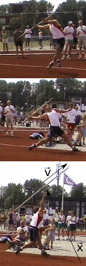
Figure 1.1: Initial conditions for throwing a javelin, cf. Example 1.2.
Example 1.2 Throwing a javelin The ICs for the flight of a javelin specify where it is released, $\mathbf x_0$, when it is thrown, the velocity $\mathbf v_0$ at that point of time, and the orientation of the javelin. In a good trial the initial orientation of the javelin is parallel to its initial velocity $\mathbf v_0$, as shown in Figure 1.1.
Remark.
In repeated experiments the ICs will be (slightly) different,
and one observes different trajectories.
1. A seasoned soccer player will hit the goal in repeated kicks.
However, even a professional may miss occasionally.
2. A bicycle involves a lot of mechanical pieces that work together to provide a predictable riding experience.
3. A lottery machine involves a smaller set of pieces than a bike,
but it is constructed such that unnoticeably small
differences of initial conditions give rise to noticeably different outcomes.
The outcome of the lottery can not be predicted,
in spite of best efforts to select identical initial conditions.
Definition 1.7 Constant of Motion
A function of the positions $\mathbf x_i$ and velocities $\mathbf v_i$ is called a constant of motion,
when it does not evolve in time.
Remark. For a given initial conditions a constant of motion takes the same value for the full trajectory. However, it may take different values for different trajectories, i.e. different choices of initial conditions.
Example 1.3 Length of a piece of chalk
During the flight the positions $\mathbf x_1$ and $\mathbf x_2$ of the piece of chalk will change.
However, the length $L$ of the piece of chalk will not,
and at any given time it can be determined from $\mathbf x_1$ and $\mathbf x_2$.
Hence, $L$ is a constant of motion that takes the same value for all trajectories of the piece of chalk.
Example 1.4 Energy conservation for the piece of chalk
We will see that the sum of the potential and the kinetic energy is conserved during the flight of the piece of chalk.
This sum, the total energy $E$, is a constant of motion.
The potential energy depends on the position and the kinetic energy is a function of the velocity.
Trajectories that start at the same position with different speed will therefore have different total energy.
Hence, $E$ is a constant of motion that can take different value for different trajectories of the piece of chalk.
Definition 1.8 Parameter
In addition to the ICs the trajectories will depend on parameters of the system.
Their values are fixed for a given system.
Example 1.5 A piece of chalk
For the piece of chalk the trajectory will depend on whether the hall is the Theory Lecture Hall in Leipzig,
a briefing room in a ship during a heavy storm,
or the experimental hall of the ISS space station.
To the very least one must specify how the gravitational acceleration acts on the piece of chalk,
and how the room moves in space.
Remark. The set of parameters that appear in a model depends on the choices that one makes upon setting up the experiment. For instance * Beckham's banana kicks can only be understood when one accounts for the impact of air friction on the soccer ball. * Air friction will not impact the trajectory of a small piece of talk that I throw into the dust bin. By adopting a clever choice of the parameterization the trajectory of the piece of chalk can be described in a setting with $5$ DOF. The length of the piece of chalk will appear as a parameter in that description.
Definition 1.9 Physical Quantities
Positions, velocities and parameters are physical quantities
that are characterized by at least one number and a unit.
Example 1.6 Physical Quantities
1. The mass, $M$, of a soccer ball can be fully characterized by a number and the unit kilogram (kg), e.g. $M \approx 0.4\,\text{kg}$.
2. The length, $L$, of a piece of chalk can be fully characterized by a number and the unit meter (m), e.g. $L \approx 7 \times 10^{-2}\,\text{m}$.
3. The duration, $T$, of a year can be characterized by a number and the unit second, e.g. $T \approx \pi\times \times 10^{7}\,\text{s}$.
4. The speed, $v$, of a car can be fully characterized by a number and the unit, e.g. $v \approx 42\,\text{km/h}$.
5. A position in a $D$-dimensional space can fully be characterized by $D$ numbers and the unit meter.
6. The velocity of a piece of chalk flying through the lecture hall can be characterized by three numbers and the unit m/s.
However, one is missing information in that case about its rotation.
Remark. Analyzing the units of the parameters of a system provides a fast way to explore and write down functional dependencies. When doing so, the units of a physical quantity $Q$ are denoted by $[Q]$. For instance for the length $L$ of the piece of chalk, we have $[L]=\text{m}$. For a dimensionless quantity $d$ we write $[d] = 1$.
Example 1.7 Changing units
Suppose we wish to change units from km/h to m/s.
A transparent way to do this for the speed of the car in the example above is by multiplications with one
\begin{align*}
v = 72 \frac{\text{km}}{\text{h}} \: \frac{ 1\,\text{h} }{3.6 \times 10^{3}\,\text{s}} \; \frac{ 1 \times 10^{3}\,\text{m} }{1\,\text{km}}
= \frac{72}{3.6} \text{m/s}
= 20\,\text{m/s}
\end{align*}
Definition 1.10 Dynamics
The characterization of all possible trajectories for all admissible ICs is called dynamics of a system.
Self Test
Problem 1.1:
The degrees of freedom of a frisbee
- How would you describe the position of a frisbee in space?
- How many degrees of freedom does your parameterization involve?
- Are there constants of motion in your description?
- Specify at least three parameters required for the description.
Problem 1.2:
Useful numbers and unit conversions
- Verify that
- one nano-century amounts to $\pi$ seconds,
- a colloquium talk at our Physics Department must not run take longer than a micro-century,
- a generous thumb-width amounts to one atto-parsec.
- The Physics Handbook of Nordling and Österman (2006)2) defines a beard-second, i.e., the length an average beard grows in one second, as $10\,\text{nm}$. In contrast, Google Calculator uses a value of only $5\,\text{nm}.$ I prefer the one where the synodic period of the moon amounts to a beard-inch. Which one will that be?
- In the furlong–firkin–fortnight (FFF) unit system one furlong per fortnight amounts to the speed of a tardy snail (1 centimeter per minute to a very good approximation), and one micro-fortnight was used as a delay for user input by some old-fashioned computers (it is equal to $1.2096\,\text{s}$). Use this information to determine the length of one furlong.