Problem 2.27: Tackling tackles and pulling pulleys

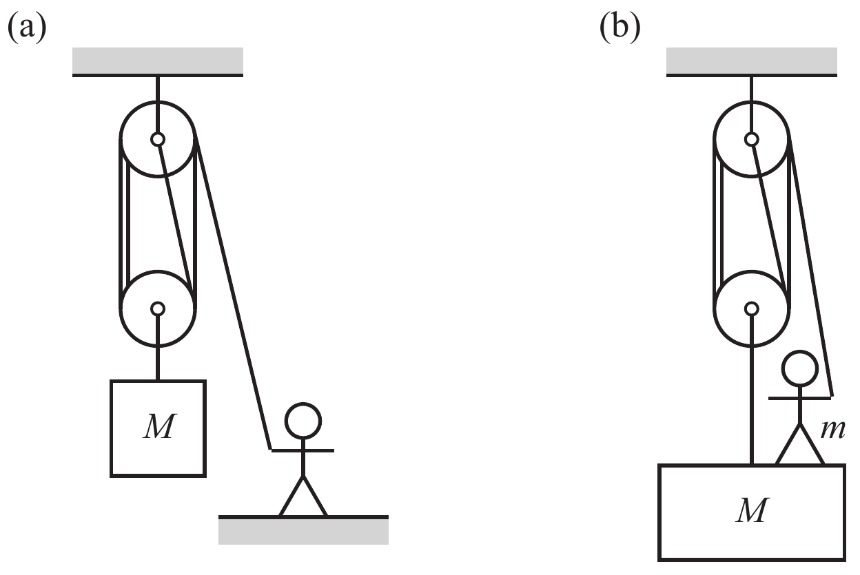
1. Which forces are required to hold the balance in the left and the right sketch?
2. Let the sketched person and the weight have masses of $m=75\text{kg}$ and $M=300\text{kg}$, respectively. Which power is required then to haul the line at a speed of $1 m/s$.

Hint: $\quad$ The power is defined here as the change of $Mg\, z(t)$ and $(M+m)\,g\,z(t)$, per unit time, respectively. Verify by dimensional analysis that this is a meaningful definition.

Problem 2.28: Angles between three balanced forces

We consider three masses $m_1$, $m_2$, and $m_3$. With three ropes they are attached to a ring at position $\mathbf q_0$. The ropes with the attached masses hang over the edge of a table at the fixed positions $\mathbf q_1 = (x_1 , \, 0)$, $\mathbf q_2 = (0 , \, y_2)$, and $\mathbf q_3 = (w, \, y_3)$. Here, $w$ denotes the width of the table board. We now determine the angles $\theta_{ij}$ between the ropes from $\mathbf q_0$ to $\mathbf q_i$ and $\mathbf q_j$, respectively.

a) Let $\hat{\boldsymbol e}_i = (\mathbf q_i - \mathbf q_0) / |\mathbf q_i - \mathbf q_0|$ be the unit vectors pointing from the ring to the positions where the ropes hang over the table edge, and $\theta_{ij}$ be the angle between $\hat{\boldsymbol e}_i$ and $\hat{\boldsymbol e}_j$. Argue why \begin{align*} \mathbf 0 = \sum_{i=1}^3 m_i \, \hat{\boldsymbol e}_i \end{align*} Multiplying this equation with $\hat{\boldsymbol e}_1$, $\dots$ $\hat{\boldsymbol e}_3$ provides three equations that are linear in $\cos \theta_{ij}$. The first one is $ 0 = M_1 + M_2 \, \cos\theta_{12} + M_3 \, \cos\theta_{13}$. Find the other two equation, and solve the equations as follows.

From the equation that is given above you find $\cos\theta_{12}$ in terms of $\cos\theta_{13}$.

Inserting this into the other equation involving $\cos\theta_{12}$ (and rearranging terms) provides $\cos\theta_{23}$ in terms of $\cos\theta_{13}$.

Inserting this into the third equation provides \begin{align*} \cos\theta_{13} = \frac{M_2^2 - M_1^2 - M_3^2}{2 \, M_1 \, M_3} \end{align*}

b) Which angle $\theta_{23}$ do you find when $M_1 = M_2 = M_3$? The three forces have the same absolute value in this case. Which symmetry argument does then also provide the value of the angle?

c) Determine also the other two angles $\theta_{13}$ and $\theta_{12}$. They can also be found from a symmetry argument without calculation.

Hint: The angles do not care which mass you denote as $1$, $2$, and $3$.

d) Note that we found the angles $\theta_{ij}$ without referring to the positions $\mathbf q_1$, $\dots$ $\mathbf q_3$! Make a sketch what this implies for the position of the ring, and how $\mathbf q_0$ changes qualitatively upon changing a mass.

e) The calculation of the position $\mathbf q_0$ can then be attacked by observing that \begin{align*} \mathbf q_0 = \mathbf q_1 + l_1 { \cos\beta \choose \sin\beta } = \mathbf q_2 + l_2 { \sin\alpha \choose -\cos\alpha } = \mathbf q_3 + l_3 {-\sin\gamma \choose -\cos\gamma } \end{align*} where $l_i$ is the distance of the ring to the position where rope $i$ hangs over the table. Further, the fact that the angles of quadrilaterals add to $2\pi$ provides \begin{align*} \alpha = \theta_{23} - \gamma \qquad\text{and}\qquad \beta = \frac{3\pi}{2} - \gamma - \theta_{13} \end{align*} Altogether these are $8$ equations to determine the two components of $\mathbf q_0$, $l_1$, $\dots$ $l_3$, and the angles $\alpha$, $\beta$ and $\gamma$. Determine $\mathbf q_0$.

Problem 2.29: Torques acting on a ladder

Figure 2.27 shows the setup of a ladder leaning to a wall. The indicated angle from the downwards vertical to the ladder is denoted as $\theta$. There is a gravitational force of magnitude $Mg$ acting of a ladder of mass $M$. At the point where it leans to the wall there is a normal force $\mathbf N$ acting from the wall to the ladder. At the ladder feet there is a normal force to the ground $\vec f$, and a tangential friction force of magnitude $\gamma_1 f$.

1. In principle there also is a friction force $\gamma_2 \, N$ acting at the contact from the ladder to the wall. Why is it admissible to neglect this force?
   Remark: There are at least two good arguments.
2. Determine the vertical and horizontal force balance for the ladder. Is there a unique solution?
3. The feet of the ladder start sliding when $\gamma_1 f$ exceeds the maximum static friction force $\gamma_s f$. Which constraints do the force balance and this condition entail for the angles $\theta$ where the ladder leans at the wall?
4. Where does the mass of the ladder enter the discussion? Do you see why?
5. Determine the torque acting on the ladder. Does it matter whether you consider the torque with respect to the contact point to the wall, the center of mass, or the foot of the ladder?
6. Determine the threshold of sliding based on the balance of torques.
   For metal feet on a wooden ground it takes a value of $\gamma_s \simeq 2$. For a slippery smooth ground it can be as small as $\gamma_s \simeq 0.3$. What does that tell about the range angles where the ladder starts to slide?
7. Why does a ladder commonly start sliding when when a man has climbed to the top? Is there anything one can do against it? Is that even true, or just an urban legend?

Problem 2.30: Walking a yoyo

The sketch to the right shows a yoyo of mass $m$ standing on the ground. It is held at a chord that extends to the top right. There are four forces acting on the yoyo: gravity $m \mathbf g$, a normal force $\mathbf N$ from the ground, a friction force $\mathbf R$ at the contact to the ground, and the force $\mathbf F$ due to the chord. The chord is wrapped around an axle of radius $r_1$. The outer radius of the yoyo is $r_2$.

1. Which conditions must hold such that there is no net force acting on the center of mass of the yoyo?
2. For which angle $\theta$ does the torque vanish?
3. Perform an experiment: What happens for larger and for smaller angels $\theta$? How does the yoyo respond when fix the height where you keep the chord and pull continuously?

Problem 2.31: Retro-reflector paths on bike wheels

The more traffic you encounter when it becomes dark the more important it becomes to make your bikes visible. Retro-reflectors fixed in the sparks enhance the visibility to the sides. They trace a path of a curtate trochoid that is characterized by the ratio $\rho$ of the reflectors distance $d$ to the wheel axis and the wheel radius $r$. A small stone in the profile traces a cycloid ($\rho=1$). Animations of the trajectories can be found at https://en.wikipedia.org/wiki/Trochoid,
http://katgym.by.lo-net2.de/c.wolfseher/web/zykloiden/zykloiden.html, and in the Sage playground where it is shown how to generate the following plots:

A trochoid is most easily described in two steps: Let $\mathbf M(\theta)$ be the position of the center of the disk, and $\mathbf D(\theta)$ the vector from the center to the position $\mathbf q(\theta)$ that we follow (i.e. the position of the retro-reflector) such that $ \mathbf q(\theta) = \mathbf M(\theta) + \mathbf D(\theta) $.

a) The point of contact of the wheel with the street at the initial time $t_0$ is the origin of the coordinate system. Moreover, we single out one spark and denote the change of its angle with respect to its initial position as $\theta$. Note that negative angles $\theta$ describe forward motion of the wheel! Sketch the setup and show that \begin{align*} \mathbf M(\theta) = \begin{pmatrix} - r \theta \\ r \end{pmatrix} \, , \qquad \mathbf D(\theta) = \begin{pmatrix} - d \, \sin( \varphi + \theta ) \\ d \, \cos( \varphi + \theta ) \end{pmatrix} \, . \end{align*} What is the meaning of $\varphi$ in this equation?

b) The length of the track of a trochoid can be determined by integrating the modulus of its velocity over time, $ L = \int_{t_0}^{t} \mathrm{d} t \; \left| \dot{ \mathbf q } ( \theta(t) ) \right| $. Show that therefore \begin{align*} L = r \: \int_{0}^{\theta} \mathrm{d} \theta \: \sqrt{ 1 + \rho^2 + 2 \rho\, \cos(\varphi+\theta )} \end{align*}

c) Consider now the case of a cycloid and use $\cos(2x) = \cos^2x - \sin^2x$ to show that the expression for $L$ can then be written as \begin{align*} L = 2 \, r \: \int_{0}^{\theta} \mathrm{d} \theta \: \left| \cos\frac{\varphi+\theta}{2} \right| \end{align*} How long is one period of the track traced out by a stone picked up by the wheel profile?

Problem 2.32: The natural numbers modulo $n$ are a group

We consider here groups $G_n$ where the combined action of group elements can be represented as a sum of two numbers modulo $n \in \mathbb N$. In other words, for the elements of $G_n$ can be represented by the numbers $\{ 0, \dots, n-1 \}$, and for all $a,b \in G_n$ we define $a \circ b = ( a + b ) \mathrm{mod} n$.

1. Show that $G_n$ is a group.
2. Show that $G_n$ represents the rotations that interchange the vertices of a regular $n$-sided polygon.

Problem 2.33: Groups with four elements

In Problem 2.32 we encountered the group $G_n$. Here, we will study another group with four elements. The neutral element will be denoted as $n$.

1. Show that the group has at least one non-trivial element $e$ that is self-inverse, $e \circ e = n$.
   Remark: Non-trivial means here that $e \neq n$.
2. Show that the group is isomorphic to $G_4$ if there is exactly one non-trivial element that is self-inverse. In other words: the group elements can be represented in that case by the numbers $\{0, \dots, 3\}$, and the operation of the group on two of its elements yields the same result as the action of $G_4$ on the corresponding numbers.
3. Show that the group is isomorphic to $G_4$ if there is at least one element that is not self-inverse.
4. Determine the group table for the case where all group elements are self-inverse. Show that it is unique, and that it is isomorphic to the symmetry group of rectangles (cf.Problem 2.6).
5. Proof that all groups with four elements are commutative by representing the group elements in terms of generating elements. Do not refer to the group table.

Problem 2.34: Conic Sections

A conic section describes the line of intersection of a double cone $\mathsf C$ and a plane $\mathsf P$ in three dimensions. In the margin we show the shape of conic sections for different inclinations that are characterized by the eccentricity $\epsilon$. Depending on the inclination of the plane one observes

• a circle, when the axis of the cone is orthogonal to $\mathsf P$, i.e. for $\epsilon=0$,
• an ellipse, when the plane is slightly tilted, $\epsilon < 1$,
• a parabola, when its inclination matches with the opening angle of the cone, $\epsilon=1$, and
• a hyperbola, when it intersects with both sides of the double cone, $\epsilon > 1$.

1. Sketch the different types of intersection of the double cone and the plane.
2. Determine the vector $\mathbf a$ that points from the vertex of the double cone to the point where the plane intersects the axis of the double cone.
3. Describe the points in the intersection as sum of $\mathbf a$ and a vector $\mathbf b$ that lies in the plane.
4. Determine the length of the vector $\mathbf b$ as function of the angle $\theta$ that characterizes the direction of $\mathbf b$ in $\mathsf P$. How can this expression be used to plot the functions shown in Figure 2.28?

Problem 2.35: Linear dependence of three vectors in 2D

In the lecture I pointed out that every vector $\mathbf v = (v_1, v_2)$ of a two-dimensional vector space can be represented as a unique linear combination of two linearly independent vectors $\mathbf a$ and $\mathbf b$, \[ \mathbf v = \alpha \: \mathbf a + \beta \: \mathbf b \] In this exercise we revisit this statement for $\mathbb{R}^2$ with the standard forms of vector addition and multiplication by scalars.

a) Provide a triple of vectors $\mathbf a$, $\mathbf b$ and $\mathbf v$ such that $\mathbf v$ can not be represented as a scalar combination of $\mathbf a$ and $\mathbf b$.

b) To be specific we henceforth fix \[ \mathbf a = \begin{pmatrix} -1 \\ 1 \end{pmatrix} \, , \qquad \mathbf b = \begin{pmatrix} 1 \\ 1 \end{pmatrix} \, , \qquad \mathbf v = \begin{pmatrix} 2 \\ -2 \end{pmatrix} \] Determine the numbers $\alpha$ and $\beta$ such that \[ \mathbf v = \alpha \: \mathbf a + \beta \: \mathbf b \]

c) Consider now also a third vector \[ \mathbf c = \begin{pmatrix} 0 \\ 1 \end{pmatrix} \] and find two different choices for $(\alpha, \beta, \gamma)$ such that \[ \mathbf v = \alpha \: \mathbf a + \beta \: \mathbf b + \gamma \mathbf c \] What is the general constraints on $(\alpha, \beta, \gamma)$ such that $\mathbf v = \alpha \: \mathbf a + \beta \: \mathbf b + \gamma \mathbf c$.
What does this imply on the number of solutions?

d) Discuss now the linear dependence of the vectors $\mathbf a$, $\mathbf b$ and $\mathbf c$ by exploring the solutions of \[ \mathbf 0 = \alpha \: \mathbf a + \beta \: \mathbf b + \gamma \mathbf c \] How are the constraints for the null vector related to those obtained in part c)?

Problem 2.36: Algebraic number fields

Consider the set $\mathbb{K} = \mathbb{Q} + I \mathbb{Q}$ with $I^2 \in \mathbb{Q}$. We define the operations $+$ and $\cdot$ in analogy to those of the complex numbers (cf. Example 2.13): For $z_1 = x_1 + I y_1$ and $z_2 = x_2 + I y_2$ we have $x_1, y_1, x_2, y_2 \in \mathbb{Q}$ and \begin{align*} \forall z_1, z_2 \in \mathbb{K} : & z_1 + z_2 = (x_1+x_2) + I \, (y_1+y_2) \\ & z_1 \cdot z_2 = (x_1\, x_2 + I^2 \, y_1 y_2) + I \, (x_1\, y_2 + y_1 \, x_2) \\ \forall c \in \mathbb{Q} , z=(x+\mathrm{i} y) \in \mathbb{K} : & c z = c\, x + I \, y \end{align*}

1. Let $I$ be a rational number, $I \in \mathbb{Q}$. Show that $\mathbb{K} = \mathbb{Q}$.
   
2. Consider $I = \sqrt{10}$. Show that $\mathbb{K}$ is a field that is different from $\mathbb{Q}$.
   
3. Consider $I = \sqrt{8}$. In this case $\mathbb{K}$ is not a field! Why?
   
4. Find the general rule: For which natural numbers $n$ does $I = \sqrt{n}$ provide a non-trivial field?
   Remark: Non-trivial means here different from $\mathbb{Q}$.

Problem 2.37: Bases for polynomials

We consider the set of polynomials $\mathbb{P}_N$ of degree $N$ with real coefficients $p_n$, $n \in \{0, \dots, N \}$, \begin{align*} \mathbb{P}_N := \left\{ \mathbf p = \left( \sum_{k=0}^N p_k \, x^k \right) \quad\text{with } p_k \in \mathbb{R}, k \in \{0, \dots, N \} \right\} \end{align*}

a) Demonstrate that $( \mathbb{P}_N , \mathbb{R}, +, \cdot )$ is a vector space when one adopts the operations \begin{align*} \forall \quad \mathbf p = \left( \sum_{k=0}^N p_k \, x^k \right) \in \mathbb{P}_N \, , \quad \mathbf q = \left( \sum_{k=0}^N q_k \, x^k \right) \in \mathbb{P}_N \, , \text{ and } c \in \mathbb{R} \; : \\ \mathbf{p} + \mathbf{q} = \left( \sum_{k=0}^N (p_k+q_k) \, x^k \right) \quad \text{ and } \quad c \cdot \mathbf{p} = \left( \sum_{k=0}^N (c\, p_k) \, x^k \right) \, . \end{align*}

b) Demonstrate that \begin{align*} \mathbf{p} \cdot \mathbf{q} = \left( \int_0^1 \mathrm{d} x \left( \sum_{k=0}^N p_k \, x^k \right) \, \left( \sum_{j=0}^N q_j \, x^j \right) \right) \, , \\ \end{align*} establishes a scalar product on this vector space.

c) Demonstrate that the three polynomials $\mathbf b_0 = (1)$, $\mathbf b_1 = (x)$ and $\mathbf b_2 = (x^2)$ form a basis of the vector space $\mathbb{P}_2$: For each polynomial $\mathbf p$ in $\mathbb{P}_2$ there are real numbers $x_k$, $k\in\{0,1,2\}$, such that $\mathbf p = x_0 \, \mathbf b_0 + x_1 \, \mathbf b_1 + x_2 \, \mathbf b_2$. However, in general we have $x_i \neq \mathbf p \cdot \mathbf b_i$. Why is that?

Hint: $\quad$ Is this an orthonormal basis?

d) Demonstrate that the three vectors $\hat{\boldsymbol e}_0 = (1)$, $\hat{\boldsymbol e}_1 = \sqrt{3} \, (2\, x-1) $ and $\hat{\boldsymbol e}_2 = \sqrt{5} \, ( 6\, x^2 - 6\, x + 1)$ are orthonormal.

e) Demonstrate that every vector $\mathbf p \in \mathbb{P}_2$ can be written as a scalar combination of $( \hat{\boldsymbol e}_0, \hat{\boldsymbol e}_1, \hat{\boldsymbol e}_2 )$, \begin{align*} \mathbf p = ( \mathbf p \cdot \hat{\boldsymbol e}_0 ) \, \hat{\boldsymbol e}_0 + ( \mathbf p \cdot \hat{\boldsymbol e}_1 ) \, \hat{\boldsymbol e}_1 + ( \mathbf p \cdot \hat{\boldsymbol e}_2 ) \, \hat{\boldsymbol e}_2 \, . \end{align*} Hence, $( \hat{\boldsymbol e}_0, \hat{\boldsymbol e}_1, \hat{\boldsymbol e}_2 )$ form an orthonormal basis of $\mathbb{P}_2$.

f) Find a constant $c$ and a vector $\hat{\boldsymbol n}_1$, such that $\hat{\boldsymbol n}_0 = (c \, x)$ and $\hat{\boldsymbol n}_1$ form an orthonormal basis of $\mathbb{P}_1$.

Problem 2.38: Systems of linear equations

A system of $N$ linear equations of $M$ variables $x_1$, $\dots$ $x_M$ comprises $N$ equations of the form \begin{align*} b_1 &= a_{11} \, x_1 + a_{12} \, x_2 + \dots + a_{1M} \, x_M \\ b_2 &= a_{21} \, x_1 + a_{22} \, x_2 + \dots + a_{2M} \, x_M \\ \vdots & \qquad \vdots \\ b_N &= a_{N1} \, x_1 + a_{N2} \, x_2 + \dots + a_{NM} \, x_M \end{align*} where $b_i, a_{ij} \in \mathbb{R}$ for $i \in \{ 1, \dots, N \}$ and $j \in \{ 1, \dots, M\}$.

a) Demonstrate that the linear equations $( \mathbb{L}_M , \mathbb{R}, +, \cdot )$ form a vector space when one adopts the operations \begin{align*} \forall \quad & \mathbf p = \bigl[ p_0 = p_{1} \, x_1 + p_{2} \, x_2 + \dots + p_{M} \, x_M \bigr] \in \mathbb{L}_N \, , \\ & \mathbf q = \bigl[ q_0 = q_{1} \, x_1 + q_{2} \, x_2 + \dots + q_{M} \, x_M \bigr] \in \mathbb{L}_N \, , \\ & c \in \mathbb{R} \; : \\ \mathbf{p} + \mathbf{q} &= \bigl[ p_0+q_0 = (p_1+q_1) \, x_1 + (p_2+q_2) \, x_2 + \dots + (p_M+q_M) \, x_M \bigr] \\ c \cdot \mathbf{p} &= \bigl[ c\, p_0 = c\,p_1 \, x_1 + c\,p_2 \, x_2 + \dots + c\,p_M \, x_M \bigr] \, . \end{align*} How do these operations relate to the operations performed in Gauss elimination to solve the system of linear equations?

b) The system of linear equations can also be stated in the following form \begin{align*} \begin{pmatrix} b_1 \\ b_2 \\ \vdots \\ b_N \end{pmatrix} &= \begin{pmatrix} a_{11} \\ a_{21} \\ \vdots \\ a_{N1} \end{pmatrix} \, x_1 + \begin{pmatrix} a_{12} \\ a_{22} \\ \vdots \\ a_{N2} \end{pmatrix} \, x_2 + \dots + \begin{pmatrix} a_{1M} \\ a_{2M} \\ \vdots \\ a_{NM} \end{pmatrix} \, x_M \\ \Leftrightarrow\qquad \mathbf b &= x_1 \: \mathbf a_1 + x_2 \: \mathbf a_2 + \dots + x_M \: \mathbf a_M \end{align*} where $\mathbf b$ is expressed as a linear combination of $\mathbf a_1$, $\dots$ $\mathbf a_M$ by means of the numbers $x_1$, $\dots$, $x_M$. What do the conditions on linear independence and representation of vectors by means of a basis tell about the existence and uniqueness of the solutions of a system of linear equations?

Problem 2.39: Crossing a river

A ferry is towed at the bank of a river of width $B=100\;$m that is flowing at a velocity $v_F = 4\;$m/s to the right. At time $t=0\;$s it departs and is heading with a constant velocity $v_B = 10\;$km/h to the opposite bank.

1. When will it arrive at the other bank when it always heads straight to the other side? (In other words, at any time its velocity is perpendicular to the river bank.) How far will it drift downstream on its journey?
2. In which direction (i.e. angle of velocity relative to the downstream velocity of the river) must the ferryman head to reach exactly at the opposite side of the river? Determine first the general solution. What happens when you try to evaluate it for the given velocities?

Problem 2.40: Piling bricks

At Easter and Christmas Germans consume enormous amounts of chocolate. If you happen to come across a considerable pile of chocolate bars (or beer mats, or books, or anything else of that form) I recommend the following experiment:

1. We consider $N$ bars of length $l$ piled on a table. What is the maximum amount that the topmost bar can reach beyond the edge of the table.
2. The sketch above shows the special case $N=4$. However, what about the limit $N \to \infty$?

Problem 2.41: Where does the bike go?

Consider the picture of the bicycle to the left. The red arrow indicates a force that is acting on the paddle in backward direction.
Will the bicycle move forwards or backwards? Take a bike and do the experiment!

Problem 2.42: Hypotrochoids, roulettes, and the Spirograph

A roulette is the curve traced by a point (called the generator or pole) attached to a disk or other geometric object when that object rolls without slipping along a fixed track. A pole on the circumference of a disk that rolls on a straight line generates a cycloid. A pole inside that disk generates a trochoid. If the disk rolls along the inside or outside of a circular track it generates a hypotrochoid. The latter curves can be drawn with a spirograph, a beautiful drawing toy based on gears that illustrates the mathematical concepts of the least common multiple (LCM) and the lowest common denominator (LCD).

1. Consider the track of a pole attached to a disk with $n$ cogs that rolls inside a circular curve with $m>n$ cogs. Why does the resulting curve form a closed line? How many revolutions does the disk make till the curve closes? What is the symmetry of the resulting roulette? (The curves to the top left is an examples with three-fold symmetry, and the one to the bottom left has seven-fold symmetry.)
2. Adapt the description for the curves developed in Problem 2.31 such that you can describe hypotrochoids.
3. Test your result by writing a Python program that plots the curves for given $m$ and $n$.